
The Influence of Interactive Videodisc Instruction Using Simultaneous-Time Analysis on Kinematics Graphing Skills of High School Physics Students
John Brungardt and Dean A. Zollman
Department of Physics, Kansas State University, Manhattan, Kansas 66506-2601
(Published in The Journal of Research in Science Teaching 32(8) 855-869 (1995))
Abstract
Real-time kinematical analysis of physical phenomenon is the graphing of displacement, velocity, and acceleration versus time data simultaneously with the motion of the object. Brasell (1987) found that students using real-time analysis with microcomputer-based laboratory (MBL) tools significantly improved their kinematics graphing skills as compared to students using delayed-time graphing (kinematics graphs produced after the motion of the object). However, Beichner (1990), using computer reanimation of videotaped images, found no difference in student learning between the simultaneous-time (kinematics graphs produced simultaneously with the motion of the image of the object, such as a video-recorded image or a computer re-animated image) and the delayed-time treatments. This investigation considers student analysis of videodisc recorded images, with treatments over an extended time. Using quantitative, qualitative and retention data, we find no significant learning difference between using simultaneous-time and delayed-time analysis for student understanding of kinematics graphs. However, the results imply that simultaneous-time analysis may have advantages in some areas.
Introduction
Graphing skills are essential if the general population is to be able to understand scientific and other information. Thus, graphing skills have been studied extensively. Recent studies have described general research efforts in the area of graphing, both of scientific data and of data from other areas (Jackson, Edwards, & Berger, 1993; Leinhardt, Zaslavsky, & Stein, 1990; Padilla, McKenzie, & Shaw, 1986). In recent years microcomputer-based laboratory (MBL) tools have been used to help teach graphing skills (Adams & Shrum, 1990; Linn, Layman, & Nachmias, 1987; Mokros & Tinker, 1987; Nachmias & Linn, 1987; Thornton, 1987; Thornton & Sokoloff, 1990). Students collect data using sensors which are connected to a small computer. As these data are collected, graphs appear, in real-time, on the computer screen. While the MBL system was originally designed to teach physics, it has shown some success in helping students to learn graphing. Most of this work has focused on the domain of kinematics. Other techniques, such as pencil-paper graphing or computer simulation, have also investigated student understanding of kinematics graphing (Goldberg & Anderson, 1989; McDermott, Rosenquist, & van Zee, 1987; Rosenquist & McDermott, 1987; Trowbridge & McDermott, 1980, 1981).
From the early days of teaching with MBL tools, investigators have suspected that displaying graphs simultaneously with the collection of data was an important factor in learning. Brasell (1987) first showed evidence that this real-time nature of MBL tools improved kinematics graphing skills. However, Beichner (1990) showed with computer reanimation of videotaped images that students who viewed a kinematics graph simultaneously with the motion of the image (simultaneous-time) had no better understanding than students who viewed the graph after the event (delayed-time). Both of these studies used a one-class period treatment, used little qualitative data, and took no data on the long term retention of concepts. The present study describes an investigation of the influence on the kinematics graphing skills of high school physics students of simultaneous-time as compared to delayed-time graphing using interactive videodisc technology. In this investigation we used extended treatments, detailed interviews, and retention data.
Physics Misconceptions and Graphing Skills
Physics students have many misconceptions that they bring to the classroom. Brown (1992) uses "the term 'misconception' to refer to students' ideas which are incompatible with currently accepted scientific knowledge" (p. 17). Others use descriptors such as "naive theories" (McCloskey, 1983, p. 299), or "alternate conceptions" (Dykstra, Boyle, & Monarch, 1992, p. 615) to describe these incompatible or conflicting ideas.
Physics Education Group at the University of Washington has completed a number of studies in the area of kinematics. For example, based on student pencil/paper constructed graphs and from narrative information, McDermott et al. (1987) categorized ten difficulties students had in the graphing of kinematics data. They found that students have five difficulties in connecting graphs to physical concepts:
Additional difficulties are associated with connecting graphs to the real world:
One goal of physics instruction is to develop curricula that will overcome these commonly recognizable misconceptions. One problem is that students do not connect the physics of motion with their everyday experiences. For example, students have a cognitive difficulty with the physics concept of negative velocity, in part because a speedometer only gives them a "positive" sense of velocity. When the physics teacher insists that 20 m/s east is a positive velocity and 20 m/s west is a negative velocity, the student is confused. Goldberg and Anderson (1987) speculate that students believe negative means "a lesser quantity" or "losing something" (p. 258). Thus, students have difficulty with the vector nature of physical quantities.
Microcomputer-based Laboratory Tools
Experimental studies of microcomputer-based laboratory tools are occurring in many locations. Thornton (1987) speculated that MBL tools assist students in learning physics concepts and skills by extending the range of student investigations, providing immediate feedback of graphs in real-time, encouraging critical thinking, and reducing laborious manual data collecting and analysis. Thornton and Sokoloff (1990) further reported on the efficacy for college students of MBL instruction as compared to traditional lecture/problem solving approaches to physics. They pointed out that "MBL tools give students the opportunity to do real science" by "the creative building and testing of models to explain the world around them" (p. 865), and by understanding "the specific and familiar before moving to the more general and abstract" (p. 866).
Mokros and Tinker (1987) found positive results with middle school students using MBL tools to assist learning of graphing concepts. They suggested four reasons why MBL materials assist students in learning: "MBL uses multiple modalities; it pairs, in real-time, events with their symbolic representation; it provides genuine scientific experiences; and it eliminates the drudgery of graph production" (p. 381). One of the modalities is the use of the student's own body as the object of motion study. This kinesthetic aspect is discussed below.
Why the relative success of MBL? Linn et al. (1987) posit that students can process only a limited amount of information at a time. This cognitive capacity can be "overloaded" if there are too many concepts at once, and especially if the concepts are conflicting, such as the physicist view conflicting with the student's preconceived view of a phenomenon. They posited a "chain of cognitive accomplishments" that is "an ideal sequence of cognitive accomplishments culminating in a desired skill" (p. 246) for graphing. For example, graphical interpretation has a "graph template" as one part of its chain. Here, students form a prototype of a particular phenomenon, and then use that template for fitting a new situation into their world view (p. 247). A possible reason for the relative success of MBL tools is that they facilitate the forming of graph templates since many graphs can be viewed easily in real-time. In addition, this real-time viewing of a graph simultaneously with the motion of the object gives "memory support" to the students (p. 252). Students do not need to recall the object in their memory when they later draw a graph, because the graph is drawn as the motion occurs.
Brasell (1987) demonstrated that high school physics students had significantly better understanding of distance and velocity graphs when viewing the graph simultaneously with the motion (real-time graphing), when compared to viewing the motion followed by the graph (delayed-time graphing). Brasell used a single laboratory period as a treatment. Students who used delayed-time graphing showed significantly fewer learning gains with as little as a 20-30 second delay in displaying the graph. She posited that this time "placed an additional information-processing demand on the students" (p. 393), which led to less understanding. In addition, Brasell found real-time MBL students to be more motivated, as the "real-time graphing made the graphs appear more responsive, more manipulable, and more concrete" (p. 394). She found that the delay-time groups "appeared to be less motivated, less actively engaged, less eager to experiment, and more concerned with procedural than conceptual issues" (pp. 393-394).
Beichner (1990) studied kinematics graphing by using computer reanimation of videotaped images of the events. He described this as a visual juxtaposition, since the real object is not being viewed, but rather a computer re-animation of a videotaped image of the object. He found that students using this technique did not have significant learning gains as compared to traditional instruction. He surmised that this visual juxtaposition effect was "not the relevant variable producing the educational impact of real-time MBL" (p. 803).
Interactive Videodisc Instruction
The efficacy of interactive videodisc instruction in science education has been described for physics (Davis, 1985), biology (Lehman, 1985), and chemistry (Brooks, Lyons, & Tipton, 1985). Experimental studies have been reported for physics (Stevens, 1984), biology (Leonard, 1989, 1992), earth science (Vitale & Romance, 1992), and chemistry (Stevens, Zech, & Katkanant, 1988; Savenye & Strand, 1989). While these studies typically showed high student interest in videodisc instruction, they have not shown the efficacy of interactive videodisc instruction in graphical skills.
However, it is plausible that interactive video could improve graphing skills. An interactive videodisc system can produce a graph simultaneously with the video image of the motion of an object. The experience is not hands-on, but it can represent a realistic event to the student, for example, a basketball free-throw. This realism, i.e., an everyday life event as compared to a contrived laboratory setting, may be a factor in the motivation students have shown for videodisc technology.
A factor that might have assisted MBL students to comprehend graphs is the manipulative nature of its hands-on laboratory environment (Brasell, 1987). The student was the object under investigation in the motion detector laboratories, so the students were involved with their own Bloom's psychomotor domain, not just the cognitive and affective domains. Beichner (1990) and Mokros and Tinker (1987) surmised that this kinesthetic feedback of MBL materials is one component that contributes to its success in kinematics studies. Videodisc instruction cannot give this component; thus, it would be informative to see if simultaneous-time graphing via videodisc instruction does improve understanding.
Methods
Videodisc Environment
The Physics of Sports videodisc (Noble & Zollman, 1988) was used to present four scenes of sporting events which represented: 1) a one-dimensional, constant velocity distance runner, 2) a one-dimensional, non-zero acceleration sprinter starting from rest, 3) a one-dimensional, free falling cheerleader (traveling upwards then downwards), and 4) a two-dimensional, free-falling basketball (also traveling upwards then downwards).
Students viewed several scenes from each sporting event on the video screen, then chose a scene to analyze. To collect data they placed an acetate sheet on the video screen, and marked the position of the image on the sheet. The video sequence was then advanced two to five frames and subsequent positions of the image were marked on the sheet. Next, the students scaled the data by placing the acetate sheet on graph paper, and manually entered the position data into the spreadsheet. The software then calculated velocity and acceleration data, and displayed graphs of the kinematics variables versus time on the computer screen (a two screen system was used due to the high cost of a one-screen system).
Treatments
Whole class instruction was used to demonstrate how to use the "acetate on screen" method for data collection. Students then worked in pairs at the videodisc systems. The simultaneous-time students saw the kinematics graphs produced on the computer screen simultaneously with the motion of the image of the object (as videodisc recorded) as seen on the video screen. The delayed-time students saw the graphs produced on the computer screen after the motion of the image of the object. The time delay was several minutes. There were no other differences in the treatments.
The difference between the display of the graphs for the simultaneous-time and delayed-time groups was controlled by the computer program. For the simultaneous-time group the computer sent a command to the videodisc player to display the appropriate video frame to accompany each point on the graph. This simultaneous display was automatic. Except for "clicking to continue" the student did not need to complete any action for the video to be displayed. Likewise, the delayed-time students’ display was computer-controlled. The duration of the delay was chosen by the researchers. Again, minimal student input was necessary for the display of the video to occur.
Brief interviews were given by one researcher, the classroom teacher of the students, at the end of each treatment to generate comments about the graphs. General questions were asked, such as "tell me about the velocity versus time graph," or "what do you mean by 'negative velocity,'" to avoid "leading the student" to a particular response. A posttest of kinematic graphing was given after the four, one-class period treatments were completed. All this was completed during a three week period. Retention interviews were given to eight students three weeks after the posttest. All treatments and interviews were videotaped. The videotapes of the students were transcripted and analyzed to document the students' understanding of kinematics graphing, specifically to ascertain the differences in learning that the students in the simultaneous-time group had as compared to the students in the delayed-time group. In what areas and in what manner does simultaneous-time graphing assist student learning?
Subjects
Thirty-one high school physics students at a private high school participated in the experiment. Thirty of the students were in twelfth grade, one was in tenth grade. Previous to the research, thirty students had completed biology and chemistry. All students had completed algebra I, all but one had completed geometry, and all but three had completed algebra II. One student was dropped from the study after an extended illness during the treatment period.
Experimental Design
A posttest only, contrast group design was used. Students were randomly assigned to the experimental group, which was simultaneous-time group, and to the contrast group, which was the delayed-time group. Within each treatment group, students were randomly assigned to a partner, and these student groups were used throughout the four treatments. Since students were randomly assigned to groups, no differences in general ability were expected between groups. Student scores from the SAT and/or ACT, as well as student grades in physics confirmed this, showing no significant differences between treatment groups.
The limitations to a post-test only, contrast group design are 1) the lack of a pre-test to determine pre-treatment equivalence; here this equivalence was confirmed as stated above, 2) differential mortality may skew the groups; here only one student was dropped from the study, and 3) pre-treatment subgroups may not be formed; here, due to the small sample size, the cell size would be too small if subgroups were formed.
Performance Measures
The posttest used was the "Questions on Linear Motion" section of the test for "Tools for Scientific Thinking" (Center for Science and Mathematics Teaching, 1988). This test assesses the understanding of graphing conventions and of the relationships exhibited by graphs and has been used extensively by Thornton and Sokoloff (1990) in their MBL studies. Posttest achievement scores were analyzed with a one-way analysis of variance. The posttests were also analyzed by sub-scores of displacement questions, velocity questions, acceleration questions, and mixed questions. Since the students worked in laboratory groups of two, the posttest scores were also analyzed using student partners as the unit of analysis.
Qualitative data were obtained by analyzing videotaped recording of students during treatments, post-treatment interviews and retention interviews. These recordings were transcripted, then analyzed by the process of unitizing and categorizing as introduced by Glaser and Strauss (1967) and operationally refined by Lincoln and Guba (1985). For example, a student comment of "negative velocity means slowing down," is a unit, here a common misconception in kinematics. All units were determined, then the different types of units were categorized into themes. For example, the comment above was categorized as the theme of "difficulty with the concept of velocity." Pre-existing themes were not used, but rather the themes emerged from the data, thus the richness of the qualitative data was fully used. These data provided documentation as to what areas and in what manner the students in the two groups had misconceptions in graphing. The frequency counts within each theme were analyzed by the Mann-Whitney U statistic to determine if the results of the simultaneous-time group were significantly different than those of the delayed-time group.
Results and Discussion
The simultaneous-time group scored higher on the posttest than the delayed-time group, but not significantly higher. Table 1 shows posttest score means, standard deviations, and standard errors. Histograms of the posttest scores showed the simultaneous-time group more clustered about the mean, and the delayed-time group showed scores that were more evenly distributed. An analysis of variance demonstrated no significant differences between treatment groups (F(1,28)=0.72, p=0.404). The assumptions of parametric tests (random selection, normal distribution, and homogeneity of variance) were met in all statistical tests.
Topically split posttest questions (displacement questions, velocity questions, acceleration questions, and mixed questions) showed no significant differences. Simultaneous-time students scored slightly higher on displacement questions, velocity questions, and mixed questions. Both groups scored virtually the same on acceleration questions.
Using student groups of two as the unit of analysis, an analysis of variance on the total of the posttest scores of each pair of students showed no significant differences between the simultaneous-time group and the delayed-time group (F(1,13)=0.88, p=0.365).
An item analysis showed some differences between the simultaneous-time group and the delayed-time group. We will only discuss areas where differences were found between groups, and areas that contribute new information to the area of misconceptions in kinematics graphing. More extensive details may be found in Brungardt (1993).
|
Treatment |
n |
Mean |
SD |
SE |
|
Simultaneous time |
14 |
29.8 |
6.2 |
1.7 |
|
Delayed time |
16 |
27.3 |
9.6 |
2.4 |
The last question asked students to sketch the three kinematic graphs for the time interval zero to six seconds of a ball thrown upward, if the ball reached its peak in three seconds. No differences were found between treatment groups on the displacement versus time graph or the velocity versus time graph, but there was a notable difference between treatment groups on the acceleration versus time graph.
The acceleration versus time graphs for the ball thrown upward demonstrated a slight difference between treatment groups. The number correct was similar, with the simultaneous-time group performing somewhat better (8 of 14, 57%) than the delayed-time group (6 of 16, 36%). However, the simultaneous-time group only had one instance of the acceleration versus time graph being similar to the velocity versus time graph (1 of 14, 7%) whereas the delayed-time group had five instances of this confusion (5 of 16, 31%). Example graphs are shown in Figure 1.
The confusion of acceleration and velocity is described by Trowbridge and McDermott (1981) and the confusion of kinematics graphs of acceleration and velocity is described by McDermott et al. (1987). Trowbridge and McDermott (1981), in an example of a ball rolling upwards and downwards on an incline, found that students "expressed the belief that when the direction of motion of the ball changed, the direction of the acceleration changed, and therefore had to pass through zero" (p. 248). Thus, an acceleration graph that is shaped like a velocity graph appears reasonable to students.
Why did simultaneous-time students do somewhat better in this aspect of kinematics graphing? Perhaps the "chain of cognitive accomplishments" that Linn et al. (1987) posited for graphing is augmented by the simultaneous-time effect, especially for higher-level abstractions. The item analysis of the posttest showed that the delayed-time students did not confuse the displacement/velocity graphs which are conceptually rather concrete, while they had difficulty with the velocity/acceleration graphs which are conceptually abstract. The simultaneous-time students were more successful at higher levels of abstraction. However, caution must be used with this conclusion, because a small sample size was used.
Figure 1. Delayed-time graphs (Student 7) of velocity versus time and acceleration versus time for a ball thrown upward.
Ten recurring themes emerged from an analysis of the transcripts of the student treatments, the post-treatment interviews, and the retention interviews. The student difficulties can be categorized as misconceptions or alternate conceptions of physical phenomenon, difficulties with relating a physical event to an abstract graph, and the inability to articulate a rigorous explanation of the physics involved. These themes do not stand alone, but are usually related to other themes. Categorization of student comments into particular themes is subjective. For example, is the student comment a confusion between velocity and acceleration, or is the comment specifically a misunderstanding of acceleration? Comments that could fit into multiple categories were analyzed within the context of the student remarks to determine what the dominant misconceptions seemed to be. Many themes corroborated the findings of McDermott et al. (1987), but some are new. The themes of student comments are listed in Table 2.
The frequencies of themes, using laboratory groups of two as the unit of analysis (Table 3), were analyzed with the Mann-Whitney U statistic, which showed no statistically significant differences between the simultaneous-time group and the delayed-time group. The transcripts revealed some slight differences, which are discussed below. Examples of student comments are provided, with further details in Brungardt (1993). The retention interviews given three weeks after the posttest showed no significant differences between group.
Only the themes which showed between group differences, and themes which contribute new information to the understanding of student learning of kinematics graphs will be discussed in detail. Themes which will not be discussed here are Theme Two, viewing a graph a picture, Theme Four, difficulties with velocity, Theme Five, difficulties with acceleration, Theme Eight, ignoring graphical abstraction in favor of giving a physical description or a memorized definition, Theme Nine, references to dynamics, and Theme Ten, references to slope or calculus. Brungardt (1993) describes all the themes in detail.
Theme one—Simultaneous-time versus delayed-time differences.
Theme two—Graph as a picture error (confusion of d vs t graph with y vs x graph).
Theme three—Use of vocabulary.
Theme four—Difficulties with velocity.
Theme five—Difficulties with acceleration.
Theme six—Confusion between different types of graphs or types of physics concepts.
Theme seven—Misconceptions about shape or starting point of graph.
Theme eight—Students wanted to ignore graphical abstracts in favor of giving a physical description, or a memorized definition.
Theme nine—References to dynamics.
Theme 10—References to slope or calculus.
|
Theme |
Frequency count (mean Rank) |
Mann-Whitney U-test |
||
|
Simultaneous time (n=5) |
Delayed time (n=5) |
z |
p |
|
|
14 (6.9) |
5 (4.1) |
-1.46 |
0.144 |
|
|
|
||||
|
|
9 (5.3) |
9 (5.7) |
-0.21 |
0.835 |
|
|
19 (6.7) |
9 (4.3) |
-1.25 |
0.210 |
|
|
10 (4.7) |
13 (6.3) |
-0.84 |
0.403 |
|
|
15 (5.5) |
15 (5.5) |
0.00 |
1.000 |
|
|
23 (4.3) |
34 (6.7) |
-1.25 |
0.210 |
|
|
11 (4.8) |
17 (6.2) |
-0.73 |
0.465 |
|
|
2 (*) |
2 (*) |
* |
* |
|
|
22 (5.1) |
26 (5.9) |
-0.42 |
0.676 |
|
|
5 (3.9) |
17 (7.1) |
-1.67 |
0.095 |
|
|
179** (5.5) |
106** (3.5) |
-1.16** |
0.248** |
*Frequency count too small to use this statistic. **Simultaneous time n = 4, and delayed time n = 4 because of 1 missing data set and 1 student without a partner.
Theme One, simultaneous-time versus delayed-time differences, showed some slight differences between groups. Several students in the simultaneous-time group were motivated by the simultaneous-time effect. In addition, delayed-time students had about 45% fewer verbal comments (as measured by lines of transcripts produced, see Table 3) than the simultaneous-time students. Brasell (1987) saw a lack of motivation in the "delay-MBL groups" (delayed-time groups), noting that these groups "appeared to be less motivated, less actively engaged, less eager to experiment, and more concerned with procedural than conceptual issues" (pp. 393-394). Yet, this motivating effect did not result in significantly higher posttest scores in this study with extended interactive videodisc treatments. The following transcript demonstrates this awareness of the simultaneous-time effect, as well as an enthusiasm for it:
Note: Students are labeled with an "S" and the student number, interviewer with an "I," parenthetical comments were added by the researcher, and categorizing themes are labeled by the number in braces:
Theme One: Example 311, simultaneous-time, 1-D constant velocity, runner:
S5 Look at that. Bad! They are doing it as he is running (*{1} noting simultaneous-time effect). He's running and accelerating and decelerating. Like every time he jumps off, boom, boom, boom (*good—noting true fluctuations in graph caused by human running motion). OK, velocity vs. time.
Later, same interview:
S4,S5 I like the graph. I like the...how they had this moving while they were plotting the graph. Yeah, that was neat.
S4 Well, you can observe, um, with the way he's running how that's all measuring out on the...
S5 Yeah, like if he had a sudden acceleration for some reason, like if he decided to sprint all of a sudden.
S4,S5 You could see how it happened on the screen...you can see the difference in distance...like if he stopped all of a sudden.
The simultaneous-time effect was referred to less as the treatments continued. This implied that the students became accustomed to the simultaneous-time effect, which could imply a novelty effect in research using a one-class period treatment. In addition, simultaneous-time students were seen to have less eye movement between the computer screen and the video screen as subsequent graphs were drawn. At first, they attended to both screens, but as the velocity graph, then as the acceleration graph was drawn, they viewed the video screen less, and attended primarily to the computer screen. This result implies that students are more likely to keep a mental picture of the event during subsequent graphs, an advantage that simultaneous-time may provide. Thus, the "memory support" of the simultaneous-time environment (Linn et al., 1987, p. 252) seems not as important when viewing several graphs one after another.
Theme Three, use of vocabulary, showed students not being fluent with the vocabulary of physics. For example, the word "constant" is used for "linearly increasing" or "constant slope" by students. Students also colloquially use "up" and "down" to refer to an increase or decrease of magnitude at times, and a direction at other times. For example, one student used "up" as a direction then used "down" as a magnitude, both referring to velocity. Examples of student comments:
Theme Three: Example 1021, simultaneous-time, 1-D non-zero acceleration, sprinter:
I What'd you get for displacement?
S22 It's pretty constant (*{3} vocabulary—wrong meaning of constant).
I Displacement is constant?...What is the shape of the graph?
S22 It's an upward slant, but it's a constant, it's constantly going up (*{3} vocabulary) at the same...I mean it's not, like, connected or anything...
Theme Three: Example 1242, delayed-time, 2-D freefall, ball:
S24 It goes up for a tiny bit when he throws it. This point right here is when it reaches the peak of its arc, when it has zero velocity.
I OK, before that, what happens to the velocity?
S24 The velocity is going down (*{3} vocabulary, should say "decreasing"), because when it rises up, it's still being pulled on by gravity (*{9} dynamics).
These locutions could be understood in context, yet if upward/ downward was used for direction, and increase/decrease was used for magnitude, the resulting communication would be more specific and less ambiguous. However, attempts to do this in classroom teaching proved difficult, since up/down is such a common way to describe motion. No differences were found between simultaneous-time and delayed-time students in the use of vocabulary.
Theme Six, confusion between types of graphs or types of physics concepts, showed no significant differences between treatment groups. However, the simultaneous-time groups has slightly less of a tendency to confuse velocity and acceleration graphs (16 simultaneous-time occurrences, 27 delayed-time occurrences, Mann-Whitney U showed z=-1.36, p=0.175). This corroborates the finding from the posttest that the simultaneous-time effect may have helped students with the more abstract concepts of kinematics graphing. The following example demonstrates this misconception:
Theme Six: Example 252.8, delayed-time, retention interview, 2-D freefall, ball:
I OK. Acceleration.
S7 (indecision) Basically, the same as velocity (draws same as velocity, *{6} acceleration/velocity confusion between types of graphs).
I Why is that?
S7 Because, I'm probably wrong, but, I thought it started out at zero. But, it doesn't gain any acceleration. It's not accelerating on the way up (*{5} thinks acceleration must mean "speeding up"), it's decelerating (*some understanding here).
Misconceptions about the shape or starting point of the graph, Theme Seven, were commonly found in student comments. Some students demonstrated the misconception that graphs must start at zero, or others used discontinuities that were not physically possible, or some misstated the shape of the graph or misread the graph in other ways. Figure 2 shows a student showing acceleration to be zero at the top of the ball's path, but then he crossed out the discontinuity when he realized his error. The most common problem in this theme was that many students tended to consider every little bump on a graph as significant, ignoring the fact that irregularities in the graphs are often due to the many error sources inherent in the filming of the event, the acetate on the screen method, etc. Simultaneous-time students had four such "fluctuation" problems, and delayed-time students had eleven such errors. Possibly the simultaneous-time students, seeing the event as the graph was drawn, attach no importance to the fluctuations, since the event shows smooth motion. However, the delayed-time students may think there was such a fluctuation in the motion, thus attach meaning to the bump on the graph. This problem is reinforced by our textbooks, which invariably have perfectly smooth kinematics curves, thus a realistic curve is hard for some students to interpret. For example:
Theme 7: Example 831, simultaneous-time, 1-D freefall, cheerleader:
I OK. Tell me about acceleration.
S16 She has a negative acceleration the entire time. Which would be logical...her acceleration is the greatest at the very beginning, when the guys push her upward. And from then on, her acceleration...here she's starting here, and she's accelerating, and she's getting faster and faster...Here I think she's starting to slow down, before she goes into her flip. And then here where she starts to pull her waist up and flip, that's why I think that's steady right there. Because her waist doesn't really move much, because as she's coming down her waist is coming up. And right here, I think is a drastic drop off because both she is falling and her waist is coming in a downward motion (*{7} he's concentrating on fluctuations of the acceleration vs. time graph—problem with real analysis, not the perfect graphs you see in texts).
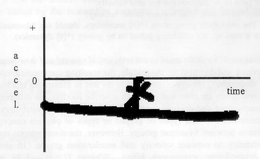
Figure 2. Simultaneous-time retention graph (Student 11) of acceleration versus time for a ball thrown upward
Conclusion
This study demonstrated, through qualitative and quantitative data, that the simultaneous-time effect is not a critical factor in improving student learning of kinematic graphing skills. However, evidence was found that the simultaneous-time effect may have some advantages in five areas: a) simultaneous-time students were aware of the simultaneous-time effect, and seemed motivated by it, b) simultaneous-time students decreased their eye movement between computer screen and video screen as subsequent graphs were produced, c) simultaneous-time students demonstrated more discussion during graphing than delayed-time students, d) simultaneous-time students displayed less confusion between velocity versus time and acceleration versus time graphs than delayed-time students, and e) simultaneous-time students did not attend to minor fluctuations in graphs as much as delayed-time students. Caution must be used due to the small sample size of this study. However, this study used an extended treatment period, so novelty effects were reduced.
The lack of greater or more significant differences could be the result of the small sample size. If one applies statistical power analysis such a the one described by Cohen (1988, pp 380-394) to this study, one finds that the probability of obtaining a statistically significant result is rather small. This analysis indicates that similar results with a larger sample size would have a much greater probability of achieving statistical significance. Thus, a large increase in the sample size could have resulted in more difference statistically than has been seen in the present work.
Two areas which impact kinematics graphing instruction were noted. First, students may be hindered in their understanding of the concept of vectors within the kinematics graphing environment by using the words up/down at times to mean a magnitude and at other times to mean a direction. The use of upward/downward for direction and increase/decrease for magnitude may help. Second, it needs to be pointed out to students that small fluctuations in a computerized graphing need not be attended to, due to errors in date collection. The overall trends must be focused on.
This study has demonstrated that the simultaneous-time effect is not a critical factor, in and of itself, of improved learning of kinematics graphing, though it may have advantages in some areas. The question remains as to why the MBL curricula is relatively successful. Further studies may investigate the kinesthetic nature of MBL tools, or other factors such as the ability of MBL tools to produce many graphs per time. Further studies in the use of videodisc technology may explore if a one-screen system would improve the visual link between the image and the graph, or if a more advanced videodisc system, capable of producing many graphs per time, would improve student learning.
References